What Statistics Is
Statistics is not a branch of mathematics that exists to punish you. It is a set of honest habits for handling one stubborn fact about the world: things vary. Two people on the same diet lose different amounts of weight, two identical machines produce slightly different parts, two polls of the same election disagree by three points. Statistics is the discipline of describing that variation clearly, and of deciding what a limited pile of data does — and does not — allow you to conclude about the much larger world it came from. This chapter builds the vocabulary that every later chapter leans on, and it does so with arithmetic no harder than what you already do to split a restaurant bill.
By the end of this chapter you can
- Explain what statistics is and why variation makes it necessary.
- Distinguish descriptive from inferential statistics and say which one a given claim uses.
- Define population, sample, parameter, and statistic, and use the correct symbols (μ, σ, N versus x̄, s, n).
- Explain why we sample, and tell sampling error apart from sampling bias.
- Classify a variable as qualitative or quantitative, and quantitative variables as discrete or continuous.
- Assign a variable to its level of measurement — nominal, ordinal, interval, or ratio — and say which calculations that level permits.
- Compute and interpret a mean, median, and range, and explain when the mean misleads.
- Read a statistical claim critically, naming the most common ways numbers are used to mislead.
Section 1Why statistics — turning data into decisions
Variation is the reason this subject exists
If every patient responded to a drug identically, you would need one patient to test it. If every light bulb failed at exactly 1,200 hours, you would need one bulb to write the warranty. Nothing behaves that way. Measurements of the same thing differ, individuals differ from one another, and repeating a study gives slightly different answers each time. Statistics is the science of collecting, organizing, summarizing, and drawing conclusions from data in the presence of that variation.
The practical payoff is decisions. A hospital deciding whether to change a protocol, a company deciding which of two web pages to keep, a city deciding where to put a bus route — all of them face the same problem. They have some data, the data are noisy, the data cover only part of the situation, and a choice still has to be made. Statistics is how you make that choice defensible rather than merely confident.
The field splits cleanly in two, and knowing which half you are in is most of the battle. Descriptive statistics summarizes the data you actually have. Inferential statistics uses those data to make a claim about a larger group you did not measure, and attaches an honest statement of uncertainty to that claim.
Descriptive statistics: making a pile of numbers speak
Suppose you record your commute, in minutes, on nine workdays:
22, 25, 19, 31, 24, 27, 21, 88, 23
Nine numbers is already too many to hold in your head. Descriptive statistics compresses them. Start with the mean (the arithmetic average), written x̄ and read “x-bar”:
x̄ = Σx ÷ n
The symbol Σ (capital sigma) just says “add them all up,” and n is how many values you have. Adding: 22 + 25 + 19 + 31 + 24 + 27 + 21 + 88 + 23 = 280, and n = 9, so
x̄ = 280 ÷ 9 = 31.1 minutes
Now the median, the middle value once the data are sorted. Sorted, the nine values are 19, 21, 22, 23, 24, 25, 27, 31, 88. With n = 9 the middle position is the 5th, so the median is 24 minutes. And the range, the crudest measure of spread, is largest minus smallest: 88 − 19 = 69 minutes.
Look at what those three numbers reveal. The mean says 31.1 minutes; the median says 24. They disagree because of a single day — the 88 — when something went badly wrong. Delete that one day and the remaining eight sum to 192, giving a mean of 192 ÷ 8 = 24.0 minutes, exactly matching the median. One unusual value dragged the average up by seven minutes. If you budgeted 31 minutes for your commute you would be early almost every single day.
That is the first real lesson of the subject: a summary is a choice, and different summaries answer different questions. The median answers “what is a typical day?” The mean answers “what happens on average over many days?” — which is the right question if you are totalling up hours lost to commuting over a year.
Inferential statistics: from the part to the whole
Descriptive work stops at the data in front of you. The moment you say “and therefore the population is like this,” you have crossed into inference. If 640 of 1,000 surveyed voters favor a measure, the descriptive fact is that 64% of those 1,000 favored it. The inferential claim — “about 64% of all voters favor it, give or take three points” — is a leap, and inference is the machinery that makes the leap safely and quantifies how far it might land off target.
Two tools do most of that work, and both are routinely misdescribed, so meet them correctly now even though the details come later. A confidence interval is a range built from your sample by a procedure with a known long-run success rate; “95% confidence” describes the procedure, meaning that if the study were repeated over and over, about 95% of the intervals produced that way would contain the true value. It does not mean there is a 95% chance that the one interval in front of you contains it. A p-value is the probability of getting data at least as extreme as yours if a specified “nothing is going on” hypothesis were true. It is emphatically not the probability that the hypothesis is true.
Both tools carry conditions, and the conditions are the part most often skipped. Their advertised performance — the 95%, the p-value — holds only if the sample was actually drawn at random from the population being described, if the observations are independent of one another, and if the model behind the calculation is a reasonable fit to the data. Feed either procedure a self-selected sample and it will still return a tidy interval and a crisp p-value; those numbers simply will not mean what they claim to. Assumptions are not fine print appended to a result. They are the load-bearing wall the result stands on, and every later chapter will state them before it states a conclusion.
| Descriptive statistics | Inferential statistics | |
|---|---|---|
| Question | What do these data look like? | What does the larger group look like? |
| Scope of claim | Only the cases measured | Beyond the cases measured |
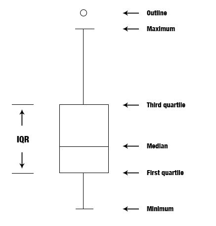
| Typical tools | Mean, median, range, standard deviation, tables, histograms, box plots | Confidence intervals, hypothesis tests, regression, margin of error |
| Uncertainty | None to report — the numbers are what they are | Must be reported — it is the whole point |
| Example | “The 30 students in this class averaged 78 on the exam.” | “Students taught this way score about 5 points higher, 95% CI 2 to 8.” |
- Statistics exists because measurements and individuals vary; its job is turning noisy data into defensible decisions.
- Descriptive statistics summarizes the data you have; inferential statistics generalizes beyond them and reports the uncertainty.
- The mean (x̄ = Σx ÷ n) is pulled by extreme values; the median is not. Report both when they disagree.
- “95% confident” describes the long-run behavior of the procedure, not the chance that this one interval is right.
Section 2Population and sample
The whole group and the piece you can afford
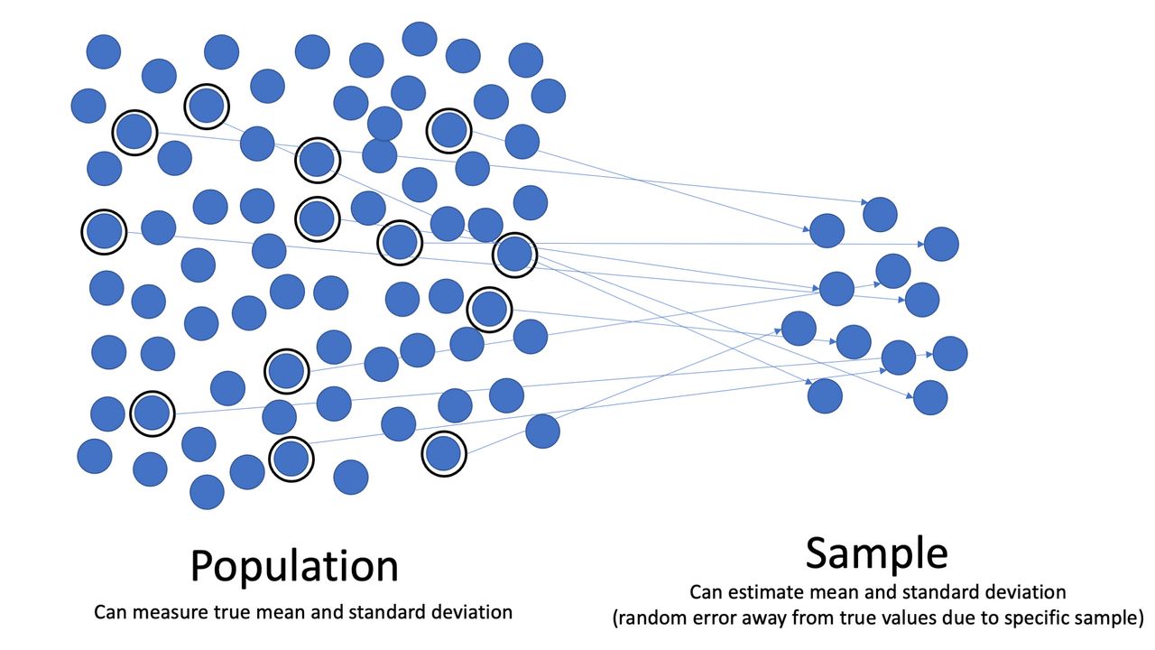
A population is the entire collection of individuals, objects, or measurements you actually want to know about. A sample is the subset of that population you manage to observe. Notice that “population” does not have to mean people: it can be every weld on a bridge, every transaction last quarter, or every possible roll of a die. What defines a population is the question you are asking. If you want to know about licensed electricians in Ohio, that is your population; a study of the electricians employed by one Ohio contractor is a sample from it, and possibly a poor one.
Measuring every member of a population is a census. It is the ideal, and it is usually impossible. Populations are too big, too expensive to reach, too spread out, still being created (next year's customers do not exist yet), or destroyed by measurement — you cannot crash-test every car you intend to sell, or taste-test every jar of sauce. A well-chosen sample of 1,200 people can describe a nation of 300 million to within a few percentage points, for the price of a few days of phone calls. That efficiency is the whole reason sampling exists.
Parameter versus statistic
This distinction carries the rest of the book, so learn it once and properly. A parameter is a number that describes a population. A statistic is a number that describes a sample. The parameter is what you want; the statistic is what you can get. Both get their own symbols, and mixing them up is the single most common notation error in a first course.
| Quantity | Population parameter | Sample statistic | Status |
|---|---|---|---|
| Size | N | n | Counts |
| Mean | μ (mu) | x̄ (x-bar) | μ is fixed and unknown; x̄ varies by sample |
| Standard deviation | σ (sigma) | s | σ is fixed and unknown; s varies |
| Proportion | p | p̂ (p-hat) | p is fixed and unknown; p̂ varies |
A memory hook that actually works: Population goes with Parameter and with Greek letters; Sample goes with Statistic and with ordinary Roman letters. Greek for the truth you cannot see, Roman for the estimate you can compute.
Worked example: one parameter, many statistics
Take a tiny population of five employees whose years of service are 2, 4, 6, 8, and 10. Because this population is small enough to measure completely, we can compute the parameter directly:
μ = (2 + 4 + 6 + 8 + 10) ÷ 5 = 30 ÷ 5 = 6 years
The population standard deviation uses σ = √[ Σ(x − μ)2 ÷ N ]. The deviations from 6 are −4, −2, 0, 2, 4; squaring gives 16, 4, 0, 4, 16, which sum to 40. So σ2 = 40 ÷ 5 = 8 and σ = √8 ≈ 2.83 years.
Now pretend we could only afford to look at three employees. Different samples of three give different answers:
| Sample of n = 3 | Sum | x̄ | Σ(x − x̄)2 | s2 = Σ(x − x̄)2 ÷ (n − 1) | s |
|---|---|---|---|---|---|
| 2, 4, 6 | 12 | 4.0 | 4 + 0 + 4 = 8 | 8 ÷ 2 = 4 | 2.00 |
| 2, 6, 10 | 18 | 6.0 | 16 + 0 + 16 = 32 | 32 ÷ 2 = 16 | 4.00 |
| 6, 8, 10 | 24 | 8.0 | 4 + 0 + 4 = 8 | 8 ÷ 2 = 4 | 2.00 |
The parameter μ never moved: it is 6, permanently. The statistic x̄ came out 4.0, 6.0, and 8.0. That spread of answers is sampling error — the unavoidable difference between a sample statistic and the population parameter that arises purely because you looked at a part instead of the whole. Sampling error is not a mistake and it cannot be eliminated, only measured and shrunk (larger samples make it smaller).
Notice also the n − 1 in the sample variance. Deviations are measured from x̄, which is itself pulled toward the sample's own values, so the squared deviations come out slightly too small on average. Dividing by n − 1 instead of n corrects that tilt, so that s2 neither systematically over- nor under-estimates σ2. Population variance divides by N; sample variance divides by n − 1.
Sampling bias is a different animal entirely. Bias is a systematic tilt in how the sample was chosen that pushes the statistic away from the parameter in a consistent direction — surveying only people who answer landlines, only customers who bothered to leave a review, only patients healthy enough to return for follow-up. The defense against sampling error is a bigger sample. The defense against bias is a properly randomized one, in which every member of the population has a known, non-zero chance of selection.
- A population is everyone or everything you want to describe; a sample is the part you observe; a census measures the whole population.
- Parameters (μ, σ, p, N) describe populations and are fixed but unknown; statistics (x̄, s, p̂, n) describe samples and change from sample to sample.
- We sample because censuses are too costly, too slow, incomplete, or destructive.
- Sampling error is the natural sample-to-sample wobble and shrinks with larger n; sampling bias is a systematic tilt from bad selection and shrinks only with better design.
Section 3Types of data
Qualitative versus quantitative
A variable is any characteristic that can differ from one individual to the next; the recorded values are the data. The first fork in the road is whether the variable names a quality or measures a quantity.
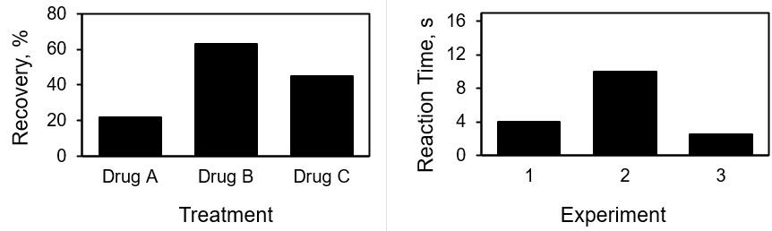
Qualitative (also called categorical) variables place each individual into a category: blood type, brand of phone, county of residence, whether a part passed inspection. The values are labels. You can count how many fall in each category and compute percentages, but the labels themselves cannot be added, averaged, or subtracted.
Quantitative (also called numerical) variables record an amount or a count: height, salary, number of siblings, reaction time in milliseconds. Their values are genuine numbers on which arithmetic means something. A useful test: if the answer to “how much” or “how many” is a number that you would meaningfully add up, the variable is quantitative.
Discrete versus continuous
Quantitative variables split again. A discrete variable can take only separated values, typically from counting — you can list the possibilities, and there are gaps between them. The number of children in a household is 0, 1, 2, 3, …; no household contains 2.4 children. A continuous variable can take any value in an interval, typically from measuring — between any two possible values there is always another. A person's weight might be 68 kg, 68.4 kg, or 68.4173 kg; the only limit is the precision of the scale.
The rule of thumb: counted things are discrete, measured things are continuous. Money is the classic gray case — strictly discrete because it comes in cents, but with so many closely spaced possible values that we treat it as continuous in practice.
| Variable | Qualitative or quantitative? | Discrete or continuous? | Why |
|---|---|---|---|
| Blood type (A, B, AB, O) | Qualitative | — | A label, not an amount |
| Eye color | Qualitative | — | A category |
| Number of siblings | Quantitative | Discrete | Counted; only whole numbers occur |
| Cars sold per day | Quantitative | Discrete | Counted; gaps between values |
| Body temperature | Quantitative | Continuous | Measured; any value in a range |
| Time to finish a race | Quantitative | Continuous | Measured; limited only by the clock |
| ZIP code | Qualitative | — | Digits used as a name for a place |
Numbers that are not quantities
Plenty of data look numeric and are not. ZIP codes, jersey numbers, patient ID numbers, and phone numbers are made of digits, but the digits function as names. The average ZIP code of your customers is a meaningless number that a spreadsheet will cheerfully compute for you. The same trap appears when categories are coded for a computer — entering 1 = single, 2 = married, 3 = divorced does not make marital status quantitative, and the “mean marital status of 1.8” is nonsense. Always ask what the number stands for, not what it looks like.
A worked point on the discrete side that trips people up: an average of a discrete variable need not be a possible value. Take five households with 1, 2, 0, 3, and 2 children. The sum is 1 + 2 + 0 + 3 + 2 = 8, and n = 5, so
x̄ = 8 ÷ 5 = 1.6 children per household
No household has 1.6 children, and that is fine. The mean is a summary of the group, not a description of any individual member. “The average family has 1.6 children” is a correct statement about families collectively and an absurd one about any family in particular.
- Qualitative (categorical) data name categories; quantitative (numerical) data measure amounts or counts.
- Quantitative data are discrete (counted, separated values) or continuous (measured, any value in an interval).
- Digits are not automatically quantities — ZIP codes and coded categories are qualitative.
- The mean of a discrete variable can be a value no individual has (1.6 children); a summary describes the group, not a member.
Section 4Levels of measurement
Four levels, each adding one property
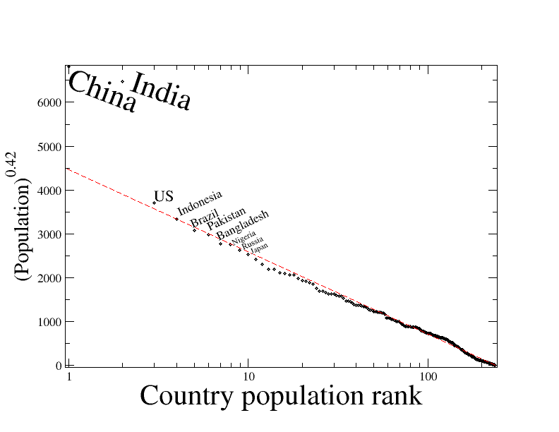
Classifying data as qualitative or quantitative is a good first cut, but it is too coarse to tell you which calculations are legitimate. The levels of measurement refine it into four rungs. Each rung keeps everything the rung below it has and adds exactly one new capability, so the ladder is easy to hold in memory.
Nominal is the bottom rung: categories with no natural order. Blood type, religion, marital status, department. You can count and compare frequencies, and that is all. The only measure of center available is the mode — the most common category.
Ordinal adds order. Categories can be ranked, but the distances between ranks are unknown or unequal. Class rank, military rank, letter grades, survey answers from “strongly disagree” to “strongly agree”, cancer stage I–IV. First, second, and third place tell you who beat whom but not by how much: the winner may have finished a tenth of a second ahead of second place and second place five minutes ahead of third. Mode and median are available; the mean is questionable.
Interval adds equal, meaningful distances. The gap between 20 and 30 is the same size as the gap between 70 and 80, so subtraction and addition are legitimate. What interval scales lack is a true zero — zero is a chosen landmark rather than the absence of the thing. Temperature in Celsius or Fahrenheit is the standard example; so are calendar years and IQ scores. Mode, median, and mean are all fair game, but ratios are not.
Ratio adds the true zero, where 0 genuinely means “none of it.” Height, weight, age, income, distance, reaction time, counts of anything. Because zero is real, ratios finally mean what they say: 40 kg is twice 20 kg, and a 60-minute task takes three times as long as a 20-minute task. Every summary statistic is permitted.
| Level | Categories? | Ordered? | Equal intervals? | True zero? | Examples | Center you may use |
|---|---|---|---|---|---|---|
| Nominal | Yes | No | No | No | Blood type, ZIP code, eye color | Mode only |
| Ordinal | Yes | Yes | No | No | Letter grade, cancer stage, race placing | Mode, median |
| Interval | Yes | Yes | Yes | No | Celsius, Fahrenheit, calendar year, IQ | Mode, median, mean |
| Ratio | Yes | Yes | Yes | Yes | Height, weight, income, time elapsed | All, plus meaningful ratios |
The zero test, worked out in numbers
The interval-versus-ratio line is the one students actually get wrong, and a single calculation settles it. Is 20°C twice as hot as 10°C? Naively 20 ÷ 10 = 2, so it looks like it. Test that claim by re-expressing the same two temperatures on a different scale and recomputing the ratio.
Convert to Fahrenheit with °F = (9 ÷ 5) × °C + 32:
10°C → (9 ÷ 5)(10) + 32 = 18 + 32 = 50°F
20°C → (9 ÷ 5)(20) + 32 = 36 + 32 = 68°F
Ratio: 68 ÷ 50 = 1.36
Convert to kelvin, which does have a true zero, with K = °C + 273.15:
10°C → 283.15 K
20°C → 293.15 K
Ratio: 293.15 ÷ 283.15 = 1.035
The same two physical states produce ratios of 2, 1.36, and 1.035 depending on which scale you happen to write them in. A quantity whose “twice as much” changes when you change units is not really a ratio at all. The kelvin figure is the honest one, because 0 K is the actual absence of thermal energy, while 0°C is just the freezing point of water — a convenient landmark someone chose. Differences, however, survive the translation perfectly: 20°C − 10°C = 10 Celsius degrees, and 293.15 K − 283.15 K = 10 kelvins. That is exactly what “interval level” means: differences are trustworthy, ratios are not.
Why the level dictates the arithmetic
Consider four patients who rate their pain on a 0–10 scale as 2, 3, 3, and 8. The mean is (2 + 3 + 3 + 8) ÷ 4 = 16 ÷ 4 = 4.0, and the median is the average of the two middle values, (3 + 3) ÷ 2 = 3.0. Which should you report? A self-reported pain rating is ordinal: nothing guarantees that the step from 2 to 3 hurts as much as the step from 7 to 8, and one patient's 8 is not another's 8. The mean of 4.0 quietly assumes equal spacing that the scale does not provide, and it has been dragged upward by the single 8. The median of 3.0 assumes only that the ratings can be ranked, which is true, so it is the safer summary.
In practice, researchers do sometimes average ordinal scales — averaging Likert responses is nearly universal — and it is often defensible when the categories are many and roughly evenly spaced. But it is a modeling assumption, not a mathematical entitlement, and it should be made knowingly. The general rule holds: statistics computed at a level higher than your data support will produce numbers that look precise and mean nothing.
- The four levels are nominal → ordinal → interval → ratio, each adding one property: order, then equal intervals, then a true zero.
- Nominal allows only counts and the mode; ordinal adds the median; interval adds the mean; ratio adds meaningful ratios.
- Interval scales lack a true zero, so 20°C is not twice as hot as 10°C — the same pair gives ratios of 2, 1.36, or 1.035 depending on the unit.
- Averaging ordinal data assumes equal spacing the scale does not guarantee; the median is the safer summary.
Section 5How statistics mislead
Correlation is not causation
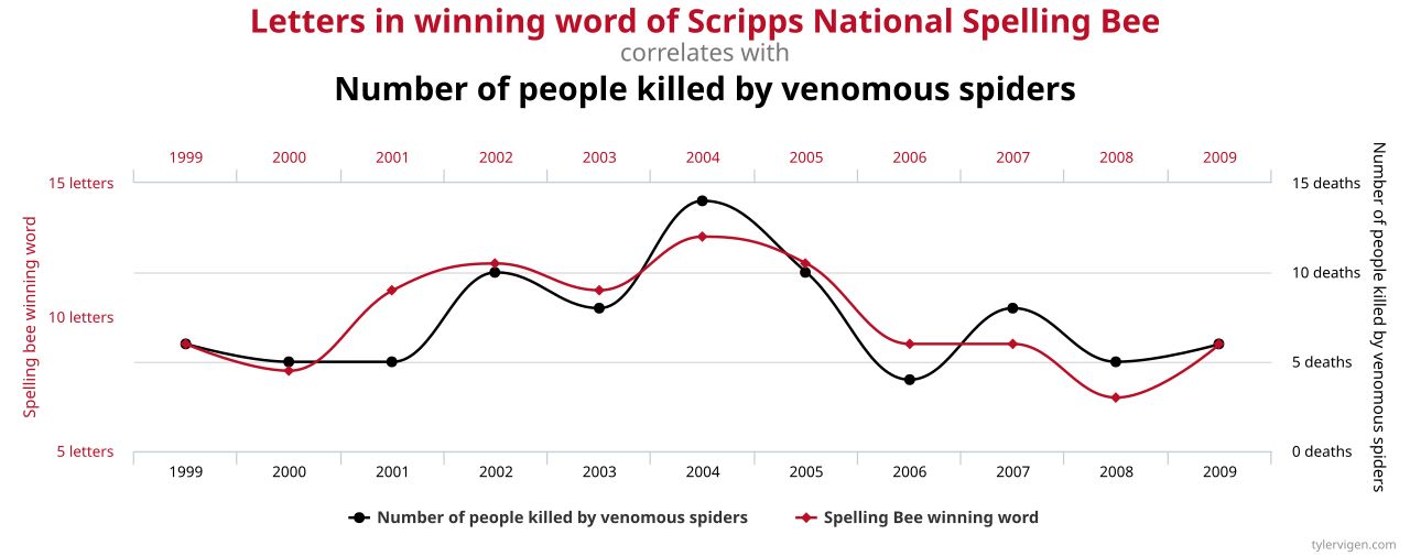
Two variables are correlated when they move together. That fact alone permits four very different explanations, and the arithmetic cannot tell them apart. A may cause B. B may cause A (hospitals are full of sick people; hospitals do not cause sickness). Some third factor — a confounding variable — may cause both. Or it may be coincidence, which is far more common than intuition suggests: sift enough series against enough other series and you will find pairs that track each other beautifully and have nothing whatever to do with one another.
The classic confounding example: ice cream sales and drownings rise and fall together across the year. Ice cream does not drown anyone. Hot weather independently drives both. The way to break a confound is a randomized experiment, in which the researcher assigns the treatment by chance so that all other factors — known and unknown — are balanced across groups on average. Observational data can suggest causes; randomization is what lets you claim one.
The standard repertoire of tricks
Most misleading statistics are not fabricated. They are true numbers presented so that a reasonable reader draws a false conclusion. A short catalogue covers most of what you will meet.
| The trick | What it looks like | The question that defeats it |
|---|---|---|
| Truncated axis | A bar chart whose y-axis starts at 94 instead of 0, turning a 2% gap into a cliff | Where does the axis start, and how big is the change really? |
| Cherry-picked window | “Crime is up 30%” measured from an unusually quiet year | Why that start date? What does the full series look like? |
| Relative risk alone | “Doubles your risk” with no baseline given | Doubles it from what to what, in absolute terms? |
| Missing denominator | “More accidents happen within 5 miles of home” | Out of how many trips? Is the rate actually higher? |
| Survivorship bias | “Our graduates earn six figures” — measured only on those who replied | Who is missing from this data, and why? |
| Average hides the spread | “Average wait 12 minutes” when half wait 2 and half wait 40 | What is the median? What is the spread? Show me the distribution. |
| Selective outcome reporting | Twenty outcomes measured, the one “significant” result published | How many things were tested? Was this planned in advance? |
| Tiny or unstated sample | “80% of users preferred it” (from ten users) | What is n? Who were they? How were they chosen? |
| Precision theater | “Satisfaction rose to 73.62%” from a survey of 200 | Do the data support that many digits? Where is the margin of error? |
The relative-risk trick deserves the arithmetic, because it is the one that changes real decisions. Suppose a condition affects 2 in 1,000 untreated people, and a new drug cuts that to 1 in 1,000. Two headlines are available, both true:
Relative risk reduction = (0.002 − 0.001) ÷ 0.002 = 0.001 ÷ 0.002 = 0.50 = 50% — “the drug halves your risk.”
Absolute risk reduction = 0.002 − 0.001 = 0.001 = 0.1 percentage points — one fewer case per thousand people treated.
From the absolute figure you get the number needed to treat: NNT = 1 ÷ 0.001 = 1,000. One thousand people must take the drug for one to benefit. “Cuts your risk in half” and “999 out of 1,000 people get no benefit” describe the identical study. Marketing prints the first; a fair report prints both. Whenever you see a percentage change in a risk, find the baseline before you react.
Reading a claim critically
You do not need advanced technique to catch most bad statistics. You need a short list of questions asked stubbornly.
- What exactly was measured, and on whom? Definitions do enormous work. “Unemployment,” “homelessness,” and “engagement” all have several defensible definitions that give different numbers.
- Who was in the sample, and how were they chosen? Volunteers, subscribers, and people who answered the phone are not random samples of anyone.
- What is n, and what is the margin of error? A result with no stated uncertainty is a result you cannot evaluate.
- Compared with what? A number without a comparison group is not evidence. “70% improved” means nothing if 70% improve without treatment.
- Is this an experiment or an observation? Only randomized assignment supports a causal claim.
- Who is missing? Dropouts, non-responders, and failed businesses are invisible in the data and often the most informative cases.
- Who paid, and what result did they want? Not disqualifying, but it tells you where to look hardest.
- Does the conclusion actually follow? Statistical significance is not practical importance; a tiny, useless effect can be “significant” in a large enough study.
Two interpretations are worth nailing down permanently, because they are misstated constantly — including in published work. A p-value of 0.03 means: if there were truly no effect, data at least as extreme as ours would occur about 3% of the time. It does not mean there is a 3% chance the effect is absent, a 97% chance the finding is real, or that the effect is large. The mirror-image error is equally common and equally damaging: a large p-value — 0.40, say — does not show that there is no effect. Failing to find convincing evidence against a hypothesis is not the same as establishing that it is true, and a small or noisy study fails to detect real effects routinely. “We did not reject it” means only that these data are compatible with it; absence of evidence is not evidence of absence. And a 95% confidence interval of 2 to 8 points describes a procedure that, used repeatedly across many studies, captures the true value about 95% of the time. For the single interval printed in front of you, the true value is either inside it or it is not; the 95% is a property of the method, not a probability attached to this one result.
- Correlation permits four explanations — cause, reverse cause, confounding, or coincidence — and only a randomized experiment singles out cause.
- Common tricks: truncated axes, cherry-picked baselines, relative risk without the absolute, missing denominators, survivorship bias, and averages that hide the spread.
- A 50% relative reduction can mean a 0.1-percentage-point absolute reduction and an NNT of 1,000. Always ask for the baseline.
- A p-value is not the probability the hypothesis is true; a 95% confidence interval describes the long-run procedure, not this one interval.
The chapter in one breath
- Statistics exists because things vary; it turns noisy, partial data into decisions you can defend.
- Descriptive statistics summarizes the data in hand; inferential statistics generalizes to a population and must report its uncertainty.
- The mean is pulled by extreme values and the median is not — nine commutes averaging 31.1 minutes had a median of just 24.
- A population is what you want to know about; a sample is what you can afford. Parameters (μ, σ, p) are fixed and unknown; statistics (x̄, s, p̂) vary from sample to sample.
- Sampling error is unavoidable wobble that shrinks with larger samples; sampling bias is a design flaw that a bigger sample does not touch — extra data only pin down the wrong value more precisely.
- Data are qualitative (categories) or quantitative, and quantitative data are discrete (counted) or continuous (measured) — digits alone do not make a quantity.
- The four levels of measurement — nominal, ordinal, interval, ratio — each add one property, and they decide which calculations are legitimate; without a true zero, “twice as much” is meaningless.
- Most misleading statistics use true numbers framed badly; ask what was measured, on whom, compared with what, out of how many, and who is missing.
ReferenceWords worth knowing
A quick reference for the terms introduced in this chapter. Skim it now to see the shape of the vocabulary, then come back whenever a word in a later chapter refuses to sit still.
- Bias (sampling bias)
- A systematic tendency for a sampling method to produce statistics that miss the parameter in a consistent direction. Unlike sampling error, it is not reduced by taking a larger sample.
- Categorical (qualitative) variable
- A variable whose values are labels placing each individual into a group, such as blood type or county. Counts and percentages are meaningful; arithmetic on the labels is not.
- Census
- A study in which every member of the population is measured, producing parameters directly rather than estimating them.
- Confidence interval
- A range of plausible values for a parameter, produced by a procedure with a stated long-run success rate. “95% confidence” describes how often the procedure captures the truth across many repetitions, not the chance that one particular interval does.
- Confounding variable
- An outside factor related to both variables under study, capable of producing a correlation between them even when neither causes the other.
- Continuous variable
- A quantitative variable that can take any value within an interval, limited only by measurement precision — height, time, temperature.
- Correlation
- A tendency for two variables to move together. A correlation is consistent with four different situations — one variable causing the other, the reverse, a confounding variable driving both, or coincidence — and the number itself cannot distinguish among them. Only a randomized experiment licenses a causal claim.
- Descriptive statistics
- Methods for organizing and summarizing the data actually collected, with no claim made about anyone not measured.
- Discrete variable
- A quantitative variable whose possible values are separated, usually arising from counting — number of children, cars sold per day.
- Inferential statistics
- Methods for drawing conclusions about a population from a sample, always accompanied by a statement of uncertainty.
- Interval level
- A level of measurement with ordered categories and equal, meaningful distances, but no true zero. Differences are meaningful; ratios are not. Celsius temperature and calendar years are examples.
- Mean
- The arithmetic average, Σx ÷ n for a sample and Σx ÷ N for a population. It uses every value, which is why a single extreme observation can pull it well away from the bulk of the data.
- Median
- The middle value of a sorted data set — the average of the two middle values when the count is even. Unaffected by how extreme the extreme values are, so it is the more honest summary of a skewed distribution.
- Mode
- The most frequently occurring value or category. The only measure of center available for nominal data.
- Nominal level
- The lowest level of measurement: unordered categories. Only counts, proportions, and the mode are meaningful.
- Ordinal level
- A level of measurement whose categories can be ranked, but with unknown or unequal distances between ranks. The median is appropriate; the mean requires an added assumption.
- Parameter
- A numerical characteristic of a population, such as μ or σ. Fixed in value and, in practice, unknown.
- Population
- The complete collection of individuals, objects, or measurements that a question is about.
- P-value
- The probability of observing data at least as extreme as those obtained, computed assuming a specified null hypothesis is true. It is not the probability that the hypothesis is true.
- Quantitative (numerical) variable
- A variable recording an amount or a count, on which arithmetic is meaningful.
- Random sample
- A sample chosen by a chance mechanism in which every member of the population has a known, non-zero probability of selection — the principal defense against bias.
- Range
- The largest value minus the smallest — the simplest measure of spread, and the most fragile, since it is determined entirely by the two most extreme observations.
- Ratio level
- The highest level of measurement: ordered, equally spaced, and possessing a true zero meaning “none.” Ratios such as “twice as much” are meaningful. Weight, income, and elapsed time are examples.
- Sample
- The subset of a population actually observed and measured.
- Sampling error
- The natural difference between a sample statistic and the population parameter, caused solely by observing a part rather than the whole. It shrinks as sample size grows.
- Statistic
- A numerical characteristic of a sample, such as x̄ or s. Computable from data, and different for every sample drawn.
- Variable
- Any characteristic that can differ from one individual to another; the recorded values of a variable are the data.