Discrete Random Variables
Up to now, probability has been about single events — one card, one coin, one roll. This chapter takes the next step: instead of asking about one outcome, we describe every outcome at once, with a number attached to each and a probability attached to each number. That package is called a probability distribution, and once you have one you can answer almost anything — how likely a result is, what to expect on average, and how far from average things typically wander. Three famous distributions do an enormous amount of the work in real life, and by the end of this chapter you will be able to recognize which one fits a situation and compute with it. None of this requires clever tricks; it requires a table, a formula, and the patience to work one line at a time.
By the end of this chapter you can
- Define a random variable and use the notation X (the variable) versus x (a value it takes).
- Classify a random variable as discrete or continuous and defend the choice.
- State the two requirements of a valid probability distribution and test a table against them.
- Compute probabilities of compound events — "at least," "at most," "more than" — from a distribution table.
- Compute the mean (μ), variance (σ2), and standard deviation (σ) of a discrete random variable, and interpret μ as a long-run average.
- State the four requirements of a binomial experiment and apply the binomial probability formula.
- Use μ = np and σ = √(npq) for a binomial, and judge whether a result is unusual.
- Recognize when the Poisson or geometric distribution applies and compute probabilities from each.
Section 1Random variables
From outcome to number
A random variable is a variable whose value is a number determined by the outcome of a chance process. That is the whole definition, and it is worth reading twice, because two ordinary words are doing precise work. Number: the result must be numeric, so if the raw outcome is "heads" or "defective," we have to convert it — count the heads, count the defects. Random: we do not know in advance which value will occur, though we may know how likely each one is.
Statisticians use a small notational habit that pays off immediately. A capital letter, usually X, names the random variable itself — the not-yet-known quantity. A lowercase letter, x, names a particular value it might take. So "X = the number of heads in three coin flips" defines the variable, and "x = 2" is one of its possible values. The expression P(X = x) then reads, in plain English, "the probability that the random variable turns out to equal this specific number." Keep the capital and lowercase straight and every formula in this chapter becomes readable.
Discrete: you can count the values
A random variable is discrete if its possible values can be listed — first value, second value, third value, and so on — with nothing squeezed in between. Counts are the classic case: the number of students absent, the number of defective units in a shipment, the number of calls arriving in an hour. You can have 3 absences or 4 absences, never 3.6.
A common misreading is that "discrete" means "only a few values." It does not. A discrete random variable may have infinitely many possible values, as long as they can be counted off in order. The number of calls arriving at a help desk in an hour could in principle be 0, 1, 2, 3, and onward forever — that list never ends, but it is still a list, so the variable is discrete. What matters is countability, not size.
Continuous: you can only measure them
A random variable is continuous if it can take any value in an interval, so that between any two possible values there is always another. Measurements behave this way: height, weight, elapsed time, temperature, blood pressure. Between 70.1 kg and 70.2 kg lies 70.15 kg, and between those lies 70.125 kg, without end.
The practical test is not "does the number have decimals?" but "was it counted or measured?" A reported time of 12.4 seconds looks like a decimal because our stopwatch stops there, but the underlying quantity is continuous — the rounding is a limitation of the instrument, not a property of the variable. Conversely, a dollar amount of $4.75 is technically discrete (money comes in cents), yet money is usually treated as continuous because the steps are so fine. Both facts can be true at once: the mathematical classification is exact, and the modeling choice is a judgment call.
| Random variable | Counted or measured? | Possible values | Type |
|---|---|---|---|
| Number of heads in 3 flips | Counted | 0, 1, 2, 3 | Discrete (finite) |
| Number of emails received today | Counted | 0, 1, 2, 3, … | Discrete (infinite but countable) |
| Number of cars in a household | Counted | 0, 1, 2, 3, … | Discrete |
| Time to finish an exam | Measured | Any value in (0, 120] minutes | Continuous |
| Weight of a cereal box | Measured | Any value near 500 g | Continuous |
| Body temperature | Measured | Any value in a range | Continuous |
- A random variable assigns a number to each outcome of a chance process; X is the variable, x is a value.
- Discrete = values can be listed (usually counts); continuous = values fill an interval (usually measurements).
- Discrete does not mean "few" — 0, 1, 2, 3, … forever is still discrete.
- For continuous variables, the probability of any single exact value is 0; we ask about intervals instead.
Section 2Probability distributions
The two rules
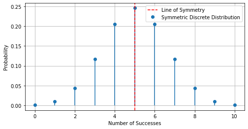
A probability distribution lists every possible value of a discrete random variable together with the probability of each. It can be written as a table, as a formula, or drawn as a probability histogram whose bar heights are the probabilities. Whatever the format, a distribution is valid only if it satisfies exactly two requirements — and these two are not arbitrary rules to memorize; each one restates something you already believe about probability.
Requirement 1: ΣP(x) = 1. The probabilities of all the values must add up to exactly 1. This says the list is complete: something has to happen, and every "something" is on the list. (In practice, allow for rounding — a table of values rounded to three decimals may total 0.999 or 1.001, and that is fine.)
Requirement 2: 0 ≤ P(x) ≤ 1 for every value x. Each individual probability must be a legitimate probability — never negative, never above 1. A single 1.4 or −0.05 anywhere in the table kills it, no matter what the total comes to.
A table fails if it breaks either rule. Suppose someone offers P(0) = 0.30, P(1) = 0.45, P(2) = 0.15. The individual values are all legal, but they sum to 0.90, so 10% of the probability has gone missing — some outcome was left off the list. Now suppose P(0) = 0.60, P(1) = 0.55, P(2) = −0.15. These do sum to 1.00, but a negative probability is meaningless, so this table is invalid too.
Reading probabilities off a distribution
Let X be the number of heads in three flips of a fair coin. The eight equally likely outcomes are HHH, HHT, HTH, THH, HTT, THT, TTH, TTT. Counting heads in each gives the distribution below, and because each of the eight outcomes has probability 1/8, the probabilities are just counts out of 8.
| x (heads) | Outcomes | P(x) as a fraction | P(x) as a decimal |
|---|---|---|---|
| 0 | TTT | 1/8 | 0.125 |
| 1 | HTT, THT, TTH | 3/8 | 0.375 |
| 2 | HHT, HTH, THH | 3/8 | 0.375 |
| 3 | HHH | 1/8 | 0.125 |
| Total | 8 outcomes | 8/8 = 1 | 1.000 |
Check the two rules: every probability sits between 0 and 1, and the total is exactly 1. Valid. Now the payoff — once a distribution is in hand, compound events are just addition, because the values are mutually exclusive.
"At most 1 head" means X = 0 or X = 1, so P(X ≤ 1) = 0.125 + 0.375 = 0.500.
"At least 2 heads" means X = 2 or X = 3, so P(X ≥ 2) = 0.375 + 0.125 = 0.500.
"At least 1 head" would mean adding 0.375 + 0.375 + 0.125 = 0.875 — but the complement is faster: P(X ≥ 1) = 1 − P(X = 0) = 1 − 0.125 = 0.875. Same answer, one subtraction.
That complement trick is worth building into your reflexes. Whenever a question says "at least one," compute 1 − P(none). With three values it saves a little effort; with a binomial of 40 trials it saves you from adding forty terms.
Filling in a missing probability
Because the probabilities must total 1, one missing entry is always recoverable. Suppose X is the number of roommates a randomly selected student has, and a survey reports P(0) = 0.15, P(1) = 0.30, P(2) = k, P(3) = 0.25, with no other values possible. Then:
0.15 + 0.30 + k + 0.25 = 1
0.70 + k = 1
k = 1 − 0.70 = 0.30
Always finish by confirming the recovered value is itself a legal probability. Here 0.30 lies between 0 and 1, so the completed table is valid. If the algebra had produced −0.10, that would not mean "probability can be negative" — it would mean the reported numbers were wrong.
- A probability distribution pairs every possible value of a discrete random variable with its probability.
- Rule 1: ΣP(x) = 1 (allowing for rounding). Rule 2: 0 ≤ P(x) ≤ 1 for every x. Both must hold.
- Compound events are found by adding the probabilities of the values they include.
- For "at least one," use the complement: P(X ≥ 1) = 1 − P(X = 0).
Section 3Expected value
The mean of a random variable is a weighted average
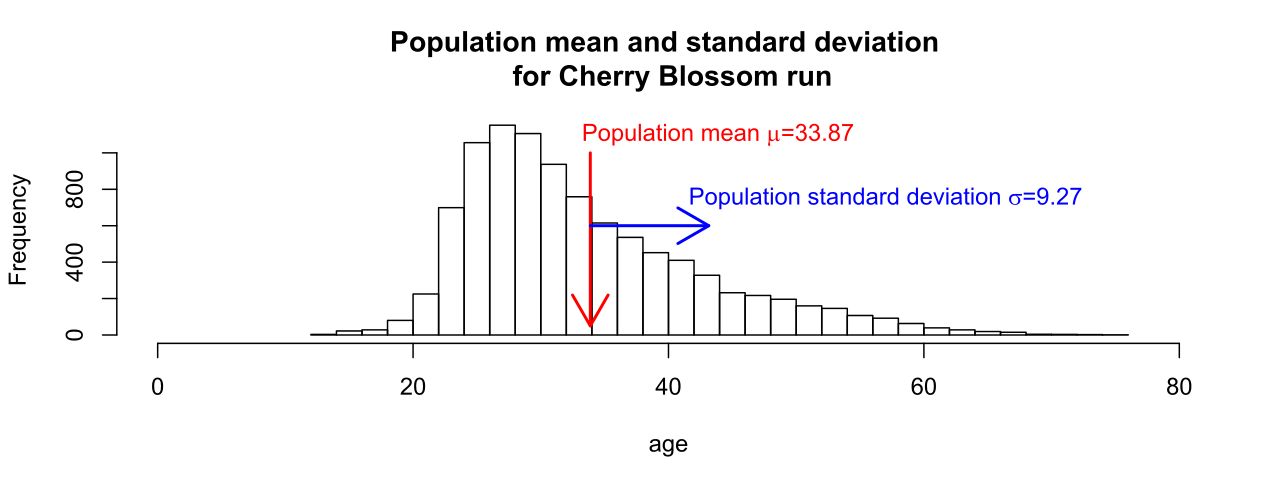
The mean of a discrete random variable, written μ and also called the expected value E(X), answers the question: if this chance process were repeated over and over, what would the average result settle down to? The formula is short:
μ = E(X) = Σ [ x · P(x) ]
Read it as an instruction: multiply each value by its probability, then add up those products. It is an average weighted by likelihood — values that happen often pull the mean toward themselves; values that happen rarely barely budge it. Notice we do not divide by anything at the end. The dividing is already built in, because the weights P(x) sum to 1.
Let X be the number of pets in a randomly selected household, with the distribution P(0) = 0.40, P(1) = 0.30, P(2) = 0.20, P(3) = 0.10. (Check: 0.40 + 0.30 + 0.20 + 0.10 = 1.00, and every entry is between 0 and 1 — valid.) Then:
μ = (0)(0.40) + (1)(0.30) + (2)(0.20) + (3)(0.10)
μ = 0 + 0.30 + 0.40 + 0.30
μ = 1.0 pet
Now the interpretation, which is where students most often go wrong. The expected value is not a prediction about the next household, and it need not even be a possible value. If the distribution had come out to μ = 1.3 pets, no household would ever own 1.3 pets; the number still describes what the average approaches across many, many households. Expected value is a statement about the long run, not about any single trial — that is the law of large numbers, and it is the whole reason insurers and casinos can plan a year in advance while having no idea what happens tonight.
Variance and standard deviation
The mean tells you where the distribution sits; it says nothing about how tightly the values cluster around it. That job belongs to the variance σ2 and the standard deviation σ. The definitional formula measures the average squared distance from the mean, again weighted by probability:
σ2 = Σ [ (x − μ)2 · P(x) ] and σ = √(σ2)
There is an algebraically identical shortcut that is far easier to compute, because it never requires subtracting the mean inside the sum:
σ2 = Σ [ x2 · P(x) ] − μ2
Both give the same answer; use whichever you find clearer. Here is the pet example carried all the way through in one table — build the columns left to right and the arithmetic takes care of itself.
| x | P(x) | x · P(x) | x2 | x2 · P(x) | (x − μ)2 · P(x) |
|---|---|---|---|---|---|
| 0 | 0.40 | 0.00 | 0 | 0.00 | (0−1)2(0.40) = 0.40 |
| 1 | 0.30 | 0.30 | 1 | 0.30 | (1−1)2(0.30) = 0.00 |
| 2 | 0.20 | 0.40 | 4 | 0.80 | (2−1)2(0.20) = 0.20 |
| 3 | 0.10 | 0.30 | 9 | 0.90 | (3−1)2(0.10) = 0.40 |
| Totals | 1.00 | μ = 1.00 | — | 2.00 | σ2 = 1.00 |
By the shortcut: σ2 = 2.00 − (1.00)2 = 2.00 − 1.00 = 1.00. By the definition, the last column also totals 1.00. The two agree, as they must. Then σ = √1.00 = 1.0 pet.
Units matter here. The variance came out in "squared pets," which means nothing to anyone, and that is precisely why we take the square root: σ is back in the original units and can be read as "a typical distance from the mean." So households average 1.0 pet, and a typical household differs from that average by about 1.0 pet.
A rough but useful convention, the range rule of thumb, treats values more than two standard deviations from the mean as unusual. Here that boundary is μ ± 2σ = 1.0 ± 2.0, an interval from −1.0 to 3.0 pets. No possible value falls outside it — 3 sits exactly on the upper boundary — so nothing in this distribution counts as unusual — which fits: a household with 3 pets is uncommon, but not startling.
Expected value as a decision tool
Expected value earns its name in situations involving money, where it tells you what a repeated bet, policy, or purchase is worth per play. Suppose a club sells 500 raffle tickets at $3 each, with one $1,000 prize. What is the expected value of buying one ticket?
Define X as your net gain, which means the $3 you paid is subtracted in both branches. If you win, you gain 1000 − 3 = $997, and that happens with probability 1/500. If you lose, you gain −$3, with probability 499/500.
E(X) = (997)(1/500) + (−3)(499/500)
E(X) = 997/500 − 1497/500
E(X) = −500/500 = −$1.00
The interpretation is exact and slightly deflating: you cannot lose exactly $1 on this raffle — you will either be up $997 or down $3 — but if you bought a ticket in this same raffle over and over, your average result would settle near a loss of $1.00 per ticket. The club's side of the same arithmetic is the mirror image: it collects $3 per ticket and pays out $1,000 spread over 500 tickets, or $2 per ticket, so it clears an average net of $1.00 per ticket — exactly what the buyer loses. (Note that $1.00 is the club's net per ticket, not its revenue; revenue is the full $3.) That balance is how the fundraiser was planned in the first place.
- μ = E(X) = Σ[x · P(x)] — a probability-weighted average; no final division is needed.
- σ2 = Σ[(x − μ)2P(x)] = Σ[x2P(x)] − μ2; then σ = √(σ2) to return to the original units.
- μ describes the long run, not the next trial, and need not be a value the variable can actually take.
- By the range rule of thumb, values outside μ ± 2σ are considered unusual.
Section 4The binomial distribution
The four requirements
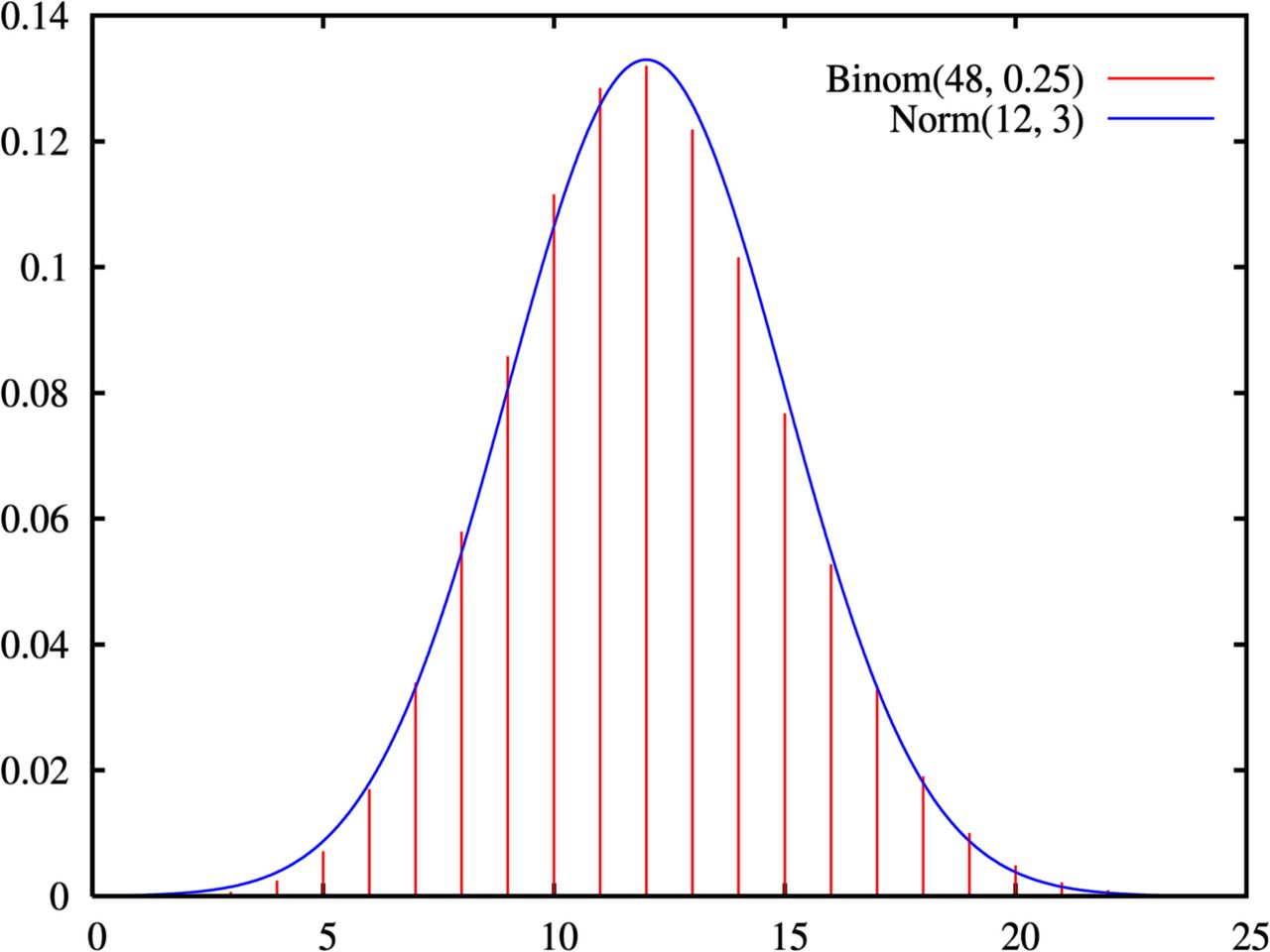
The binomial distribution is the most heavily used discrete distribution in statistics, because an enormous number of real questions have the same skeleton: we repeat something a fixed number of times, and we count how often it works. A situation qualifies as a binomial experiment only if all four of the following hold. Miss one and the formula in the next subsection gives a wrong answer.
| # | Requirement | What it means | What breaks it |
|---|---|---|---|
| 1 | Fixed number of trials | n is decided in advance and does not depend on results | "Keep testing until 3 fail" — n is not fixed |
| 2 | Two outcomes per trial | Each trial is a success or a failure — nothing else | A five-level rating scale (unless collapsed to two) |
| 3 | Independent trials | One trial's result does not change any other's probability | Drawing cards without replacement |
| 4 | Constant probability p | The success probability is identical on every trial | A test-taker who learns as the quiz goes on |
Two conventions clear up most confusion. First, "success" is just a label for the outcome you chose to count — it can be a defect, a failure, or a death. If you are counting defective parts, a defect is a "success," and p is the probability of a defect. Second, p is the probability of success on one trial, q = 1 − p is the probability of failure, and x is the number of successes in the n trials, so x can be any whole number from 0 to n.
The binomial formula
P(X = x) = nCx · px · qn−x where nCx = n! / [ x! (n − x)! ]
The formula is three ideas multiplied together, and it stops looking intimidating once you see them separately. The piece px is the probability of getting x successes; qn−x is the probability of the remaining n − x failures; multiplying them is legal precisely because the trials are independent (requirement 3). But that product is the probability of one specific arrangement, such as success-success-failure-failure. The binomial coefficient nCx counts how many arrangements produce x successes, and since each arrangement has the same probability, we multiply by that count.
Worked example. A quiz has 6 multiple-choice questions with 4 choices each. A student guesses on every question. What is the probability of exactly 2 correct?
Check the four requirements: n = 6 fixed ✓; each question is right or wrong ✓; guesses do not affect one another ✓; p = 1/4 = 0.25 on every question ✓. So n = 6, p = 0.25, q = 0.75, x = 2.
Step 1 — the coefficient: 6C2 = 6! / (2! · 4!) = (6 × 5) / (2 × 1) = 30/2 = 15.
Step 2 — the successes: (0.25)2 = 0.0625.
Step 3 — the failures: (0.75)4 = 0.31640625.
Step 4 — multiply: 15 × 0.0625 × 0.31640625 = 0.9375 × 0.31640625 = 0.2966.
So there is about a 29.7% chance of exactly 2 correct. Running the same formula for every value of x produces the complete distribution:
| x correct | 6Cx | (0.25)x(0.75)6−x | P(x) |
|---|---|---|---|
| 0 | 1 | 0.177979 | 0.1780 |
| 1 | 6 | 0.059326 | 0.3560 |
| 2 | 15 | 0.019775 | 0.2966 |
| 3 | 20 | 0.006592 | 0.1318 |
| 4 | 15 | 0.002197 | 0.0330 |
| 5 | 6 | 0.000732 | 0.0044 |
| 6 | 1 | 0.000244 | 0.0002 |
| Total | — | — | 1.0000 |
The column totals 1.0000, confirming this is a valid probability distribution — a good habit whenever you build a binomial table by hand. Compound questions now work exactly as in Section 2. "What is the probability of at least 1 correct?" Use the complement: P(X ≥ 1) = 1 − P(0) = 1 − 0.1780 = 0.8220. "At least 4 correct?" Add the tail: 0.0330 + 0.0044 + 0.0002 = 0.0376, under 4%.
Mean and standard deviation of a binomial
You could find μ and σ by running the Section 3 machinery on all seven rows — but for a binomial there are shortcuts, and they are exact, not approximations:
μ = np σ2 = npq σ = √(npq)
For the guessing student: μ = np = (6)(0.25) = 1.5 correct, which is sensible — guess on 6 questions with a 1-in-4 chance and you average one and a half. And σ = √[(6)(0.25)(0.75)] = √1.125 = 1.06 correct.
Apply the range rule of thumb: μ ± 2σ = 1.5 ± 2.12, an interval from −0.62 to 3.62. Scores of 0, 1, 2, or 3 are ordinary for a guesser; a score of 4 or more is unusual. That verdict matches the exact tail probability we just computed, P(X ≥ 4) = 0.0376. The rule of thumb and the exact calculation agree, which is the point of having both: the rule is quick, the calculation is precise.
- A binomial experiment needs all four: fixed n, two outcomes, independent trials, constant p.
- P(X = x) = nCx px qn−x — arrangements × successes × failures.
- "Success" is only a label for whatever you are counting; p must match that label.
- μ = np and σ = √(npq); sampling under 5% of a population may be treated as binomial.
Section 5Other discrete distributions
The Poisson distribution
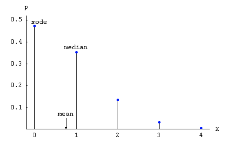
The binomial needs a fixed number of trials. But many real counts have no trials to fix: calls arriving at a help desk in an hour, typos on a page, potholes per kilometer of road. There is no n, because there is no upper limit on how many could occur. For these, the Poisson distribution models the number of events in a fixed interval of time, area, volume, or distance, given a known average rate.
P(X = x) = ( λx · e−λ ) / x! for x = 0, 1, 2, 3, …
Here λ (lambda) is the mean number of events per interval, and e ≈ 2.71828 is the natural base. The distribution needs three conditions: the events occur independently, the average rate λ is constant over the interval, and the interval is fixed. It has one striking property — a single parameter controls everything:
μ = λ σ2 = λ σ = √λ
The mean and the variance are the same number. That is a genuinely useful diagnostic: if you have count data whose sample variance is far larger than its mean, the Poisson model is probably wrong for it.
Worked example. A help desk receives an average of 3 calls per hour. What is the probability of exactly 5 calls in a given hour?
Here λ = 3 and x = 5.
Step 1: λx = 35 = 243.
Step 2: e−3 = 0.049787.
Step 3: x! = 5! = 5 × 4 × 3 × 2 × 1 = 120.
Step 4: P(X = 5) = (243 × 0.049787) / 120 = 12.0983 / 120 = 0.1008.
So about a 10.1% chance of exactly 5 calls. The chance of a completely quiet hour is P(X = 0) = (30 · e−3)/0! = 0.049787, roughly 5% — recall that 30 = 1 and 0! = 1. And the chance of at least one call is the complement: 1 − 0.0498 = 0.9502. The standard deviation is σ = √3 ≈ 1.73 calls.
One more use worth knowing: when a binomial has a large n and a small p — a common rule of thumb is n ≥ 100 and np ≤ 10 — the Poisson with λ = np closely approximates it. This is why Poisson models rare events so well: accidents at an intersection, rare defects on a production line, unusual claims filed with an insurer.
The geometric distribution
The geometric distribution flips the binomial question around. A binomial fixes the number of trials and lets the number of successes vary. A geometric fixes the number of successes at exactly one — the first one — and lets the number of trials vary. It answers: how many attempts until the first success?
P(X = x) = qx−1 · p for x = 1, 2, 3, …
The logic is transparent: to have the first success on trial x, you need x − 1 failures first (probability qx−1) followed by one success (probability p). There is no coefficient because there is only one arrangement that works. The requirements are the binomial's minus the fixed n: independent trials, two outcomes, and a constant p. Its mean and standard deviation are:
μ = 1/p σ2 = q/p2 σ = √q / p
Worked example. A representative converts 20% of the calls she makes, independently. What is the probability her first conversion comes on the 4th call?
Here p = 0.20, q = 0.80, x = 4.
P(X = 4) = (0.80)3 × 0.20 = 0.512 × 0.20 = 0.1024, about 10.2%.
How many calls does it take on average to get that first conversion? μ = 1/p = 1/0.20 = 5 calls — the reciprocal, exactly as intuition suggests. Read that carefully: μ counts the successful call itself, so the average number of failed calls preceding the first conversion is 4, not 5. The spread is σ = √0.80 / 0.20 = 0.894/0.20 = 4.47 calls, which is large relative to the mean; waiting times of this kind are notoriously variable. And the probability she needs more than 3 calls is simply the probability the first 3 all fail: P(X > 3) = (0.80)3 = 0.512. So P(X ≤ 3) = 1 − 0.512 = 0.488.
One caution when reading other sources: some define the geometric variable as the number of failures before the first success, so it starts at 0 instead of 1 and has mean q/p. The mathematics is the same; only the starting point shifts. Always check which version a formula sheet or calculator is using before plugging in.
Choosing among the three
Nearly every discrete problem you meet at this level fits one of these three, and the fastest way to identify which is to ask what is fixed and what is random.
| Distribution | What is fixed | What is random | Values of X | Mean | Variance |
|---|---|---|---|---|---|
| Binomial | Number of trials n | Number of successes | 0, 1, …, n | np | npq |
| Poisson | The interval (time, area, …) | Number of events | 0, 1, 2, … | λ | λ |
| Geometric | Number of successes (one) | Number of trials needed | 1, 2, 3, … | 1/p | q/p2 |
- Poisson: P(x) = λxe−λ/x! counts events in a fixed interval; uniquely, μ = σ2 = λ.
- Poisson approximates a binomial when n is large and p is small, using λ = np.
- Geometric: P(x) = qx−1p counts trials until the first success, with μ = 1/p.
- Identify the distribution by asking what is fixed (trials, interval, or successes) and what is random.
The chapter in one breath
- A random variable attaches a number to each outcome of a chance process; it is discrete if its values can be listed (counts) and continuous if they fill an interval (measurements).
- A probability distribution is valid only if ΣP(x) = 1 and 0 ≤ P(x) ≤ 1 for every value; both rules must hold.
- Compound events are sums of value probabilities, and "at least one" is fastest as 1 − P(0).
- The expected value μ = Σ[xP(x)] is a probability-weighted average describing the long run — not the next trial, and not necessarily a possible value.
- Spread comes from σ2 = Σ[x2P(x)] − μ2, with σ = √(σ2) restoring the original units; values beyond μ ± 2σ are conventionally called unusual.
- A binomial needs fixed n, two outcomes, independence, and constant p; then P(x) = nCxpxqn−x, μ = np, σ = √(npq).
- The Poisson counts events in a fixed interval with μ = σ2 = λ; the geometric counts trials until the first success with μ = 1/p.
- Choose a model by asking what the problem holds fixed — the trials, the interval, or the single success you are waiting for.
ReferenceWords worth knowing
A quick reference for the terms in this chapter — skim it now, or circle back whenever a word trips you up.
- Bernoulli trial
- A single trial with exactly two possible outcomes, labeled success and failure, with success probability p. A binomial experiment is n independent Bernoulli trials.
- Binomial coefficient
- The count nCx = n!/[x!(n−x)!] of the different arrangements that give x successes in n trials.
- Binomial distribution
- The distribution of the number of successes in a fixed number of independent trials with constant success probability; P(x) = nCxpxqn−x.
- Continuous random variable
- A random variable that can take any value in an interval; probabilities are assigned to intervals, and the probability of any single exact value is 0.
- Cumulative probability
- The probability that a random variable is at most a given value, P(X ≤ x), found by adding the probabilities of all values up to and including x.
- Discrete random variable
- A random variable whose possible values can be listed, such as 0, 1, 2, 3; usually the result of counting. The list may be infinite.
- Expected value
- Another name for the mean of a random variable, E(X) = μ = Σ[xP(x)]; the long-run average over many repetitions.
- Factorial
- The product n! = n(n−1)(n−2)…(1), with 0! defined as 1.
- Geometric distribution
- The distribution of the number of independent trials needed to obtain the first success; P(x) = qx−1p, with mean 1/p.
- Independent trials
- Trials in which the outcome of one has no effect on the probabilities of any other.
- Law of large numbers
- The principle that as a chance process is repeated more and more times, the average of the results converges to the expected value.
- Mean of a random variable (μ)
- The probability-weighted average of the values, Σ[xP(x)]; the balance point of the distribution.
- Memoryless property
- The feature of the geometric distribution that past failures do not change the probability of success on the next trial.
- Parameter
- A number that describes a population or a probability model, such as n and p for a binomial or λ for a Poisson.
- Poisson distribution
- The distribution of the number of events occurring in a fixed interval at a constant average rate λ; P(x) = λxe−λ/x!, with mean and variance both equal to λ.
- Probability distribution
- A listing, formula, or graph giving every possible value of a discrete random variable together with its probability.
- Probability histogram
- A bar graph of a discrete distribution in which the values sit on the horizontal axis and the bar heights are the probabilities.
- Random variable
- A variable whose numeric value is determined by the outcome of a chance process; written X, with x denoting a particular value.
- Range rule of thumb
- A rough convention that values farther than 2 standard deviations from the mean — outside μ ± 2σ — may be considered unusual.
- Standard deviation of a random variable (σ)
- The square root of the variance; a typical distance of the values from the mean, expressed in the original units.
- Success probability (p)
- The probability of the outcome being counted on a single trial; its complement q = 1 − p is the failure probability.
- Variance of a random variable (σ2)
- The probability-weighted average squared distance from the mean, Σ[(x−μ)2P(x)], equal to Σ[x2P(x)] − μ2.