Confidence Intervals
A sample can tell you what it saw, but it cannot tell you the truth about the whole population — not exactly. A confidence interval is the honest way to report that gap: instead of a single number that is almost certainly a little wrong, you report a range of plausible values, along with how confident the method is. The recipe is short enough to memorize in one line: take your best estimate and stretch it by a margin of error. This chapter builds that line from scratch, works the arithmetic for means and for proportions, shows exactly what makes an interval wide or narrow, and — the part most people get wrong — teaches you to say what “95% confident” actually means.
By the end of this chapter you can
- Explain why a point estimate alone is insufficient, and describe a confidence interval as estimate ± margin of error.
- Identify the three moving parts of every interval: the point estimate, the critical value, and the standard error.
- Build a confidence interval for a population mean using z when σ is known and t when it is not.
- State the degrees of freedom for a one-sample t interval and explain why the t distribution has heavier tails than z.
- Build a confidence interval for a population proportion and check its conditions before you trust it.
- Predict how the interval changes when the confidence level, the sample size, or the variability changes.
- Solve for the sample size needed to hit a target margin of error.
- Write a correct interpretation of a 95% confidence interval — and recognize the four classic wrong ones.
Section 1The idea of a confidence interval
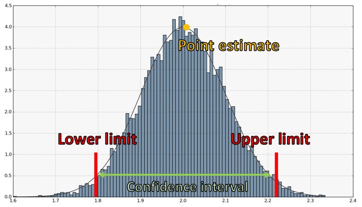
Why a single number is never enough
Suppose you want to know the average number of hours adults in a small city sleep each night. You cannot ask all 24,000 of them, so you take a random sample of 25 and compute a sample mean of 6.8 hours. That 6.8 is a point estimate: a single number, computed from a sample, offered as your best guess for the parameter — the true population mean μ, which you will never observe directly.
Here is the uncomfortable truth about point estimates: yours is almost certainly wrong. Not badly wrong, and not wrong on purpose — just wrong, because a different random sample of 25 adults would have given 7.1, and another would have given 6.5. The estimate moves around from sample to sample. That movement is called sampling error, and it is not a mistake you made; it is an unavoidable consequence of looking at a part instead of the whole.
So reporting “6.8 hours” with a straight face overstates what you know. Reporting “somewhere between 6.1 and 7.5 hours, and here is how sure I am of that method” is honest. That second statement is a confidence interval: an interval estimate for a parameter, paired with a stated confidence level.
The one-line recipe
Every confidence interval at this level — for a mean, for a proportion, for a difference between two groups — is built from the same skeleton:
point estimate ± margin of error
and the margin of error is itself always the same two things multiplied together:
margin of error = (critical value) × (standard error of the estimate)
The standard error measures how much your estimate bounces around from sample to sample — it is the standard deviation of the estimate's sampling distribution. The critical value (written z* or t*) is a multiplier chosen so that the interval is wide enough to succeed as often as your confidence level demands. Want more confidence? Use a bigger multiplier. That is the entire machine. Everything that follows in this chapter is filling in those two blanks for a specific situation.
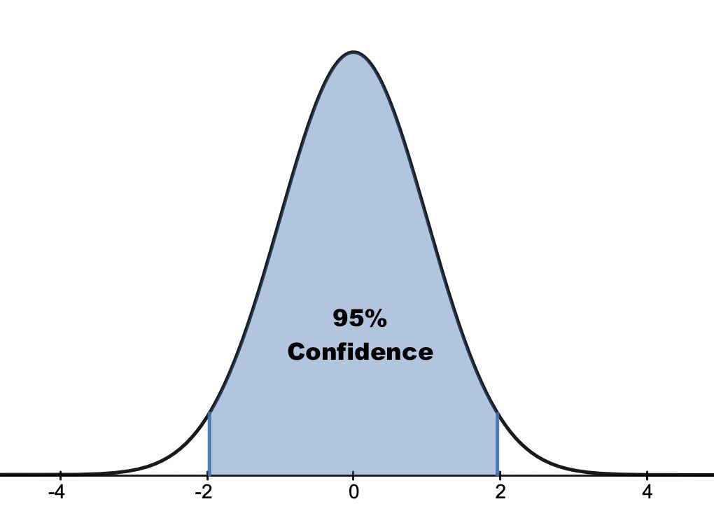
Why does this work at all? Because of the Central Limit Theorem from the previous chapters: for a large enough sample, the sampling distribution of the sample mean is approximately normal, centered on the true parameter. If the estimate lands within about 1.96 standard errors of the truth roughly 95% of the time, then reaching out 1.96 standard errors from the estimate will capture the truth roughly 95% of the time. The interval is the sampling distribution read backwards.
| Parameter (unknown) | Symbol | Point estimate | Standard error of the estimate |
|---|---|---|---|
| Population mean | μ | x̄ (sample mean) | σ/√n if σ known; s/√n if not |
| Population proportion | p | p̂ (sample proportion) | √[p̂(1 − p̂)/n] |
| Population standard deviation | σ | s (sample SD) | — (not covered here) |
| Difference of two means | μ1 − μ2 | x̄1 − x̄2 | √[s12/n1 + s22/n2] |
Reading an interval out loud
An interval has a center (your point estimate), a half-width (the margin of error), and two endpoints. If a poll reports “54% approve, margin of error 3 percentage points,” the interval is 51% to 57%, the center is 54%, and the half-width is 3. Notice that the width of the whole interval is twice the margin of error — a distinction that trips people up constantly. A margin of error of 3 points produces an interval 6 points wide.
One more habit worth building now: a confidence interval is a statement about a parameter, not about an individual. An interval of 6.1 to 7.5 hours is about the population's average sleep. It says nothing about whether any particular person sleeps in that range — most of them will not. The tool for individuals is a prediction interval, and it is much wider.
- A point estimate is a single-number guess for a parameter; it varies from sample to sample because of sampling error.
- A confidence interval is point estimate ± margin of error, reported with a stated confidence level.
- Margin of error = critical value × standard error; the standard error measures sample-to-sample bounce.
- The width of an interval is twice the margin of error, and the interval describes a parameter, never an individual.
Section 2A confidence interval for a mean
When σ is known: the z interval
Start with the easier case, the one that almost never happens in real life but makes the logic visible. Suppose the population standard deviation σ is genuinely known — a filling machine whose long-run variability the manufacturer has measured over millions of bottles, say. Then the standard error of the sample mean is exactly σ/√n, and the interval is
x̄ ± z* · (σ/√n)
where z* is the value that cuts off the middle portion of the standard normal curve matching your confidence level. For 95%, that value is 1.96 — the number worth committing to memory.
Worked example. A bottling line fills 500 mL bottles. The machine's long-run standard deviation is known to be σ = 4 mL. A quality inspector pulls a random sample of n = 36 bottles and finds x̄ = 502 mL. Build a 95% confidence interval for the true mean fill volume μ.
- Standard error: σ/√n = 4/√36 = 4/6 = 0.6667 mL
- Critical value at 95%: z* = 1.96
- Margin of error: 1.96 × 0.6667 = 1.31 mL
- Interval: 502 − 1.31 = 500.69 and 502 + 1.31 = 503.31
The 95% confidence interval is 500.69 mL to 503.31 mL. Because 500 mL falls just outside this interval, a true mean of exactly 500 mL is not among the plausible values this sample supports — the data do give evidence, at the 5% level, that the machine is off target. Notice how narrowly it misses: had the sample mean been 501 mL, the interval would have run 499.69 to 502.31 and 500 would have been comfortably inside.
When σ is unknown: the t interval
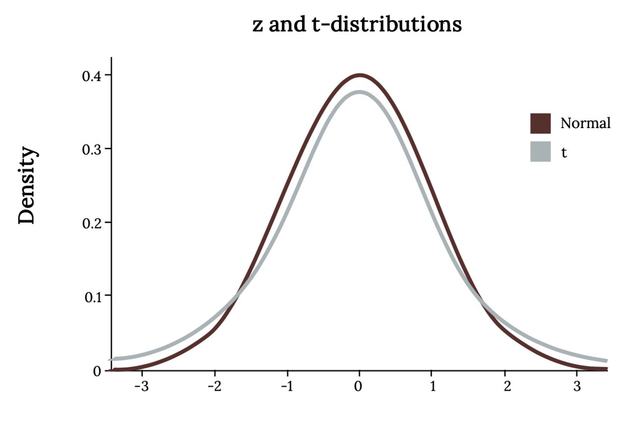
In practice you almost never know σ. You estimate it with the sample standard deviation s, which introduces a second source of uncertainty: not only is x̄ a noisy estimate of μ, but s is a noisy estimate of σ. If you simply swapped s for σ and kept using 1.96, your intervals would be a little too narrow and would capture the truth less than 95% of the time.
William Gosset solved this in 1908, publishing under the pen name “Student.” His fix was a new family of curves — Student's t distribution — that look like the normal curve but with heavier tails, which produces slightly larger critical values and slightly wider intervals. Exactly how much heavier depends on the degrees of freedom, df = n − 1. Small samples give few degrees of freedom, fat tails, and big multipliers; large samples give many degrees of freedom, and t converges on z.
x̄ ± t*n−1 · (s/√n)
Worked example. A random sample of n = 25 adults completes a reaction-time task. The sample mean score is x̄ = 78.4 with sample standard deviation s = 9.0. Build a 95% confidence interval for the population mean μ.
- Degrees of freedom: df = 25 − 1 = 24
- Standard error: s/√n = 9.0/√25 = 9.0/5 = 1.80
- Critical value: t* at 95% with df = 24 is 2.064
- Margin of error: 2.064 × 1.80 = 3.72
- Interval: 78.4 − 3.72 = 74.68 and 78.4 + 3.72 = 82.12
The 95% confidence interval is 74.68 to 82.12. Notice what the correction cost: had you carelessly used z* = 1.96, the margin would have been 3.53 and the interval 74.87 to 81.93 — noticeably too narrow, and too confident.
Conditions, and how t collapses into z
Any interval for a mean — the z version and the t version alike — rests on two assumptions, and you should state and check them before you trust the arithmetic in either worked example above. First, the data must come from a random sample (or a randomized experiment), and the observations must be independent — when sampling without replacement, a practical check is that the sample is less than 10% of the population. Second, the sampling distribution of x̄ must be roughly normal. That holds if the population itself is roughly normal, or, thanks to the Central Limit Theorem, if n is large enough (n ≥ 30 is the usual rule of thumb, and more is needed if the data are badly skewed or contain outliers).
The table below shows the 95% critical value shrinking toward 1.96 as the sample grows. This is why software uses t for everything: with n = 100 the difference between 1.984 and 1.960 is trivial, and with n = 10 it is not.
| Sample size n | df = n − 1 | t* at 95% | z* at 95% | How much wider is t? |
|---|---|---|---|---|
| 5 | 4 | 2.776 | 1.960 | +42% |
| 10 | 9 | 2.262 | 1.960 | +15% |
| 25 | 24 | 2.064 | 1.960 | +5% |
| 50 | 49 | 2.010 | 1.960 | +3% |
| 100 | 99 | 1.984 | 1.960 | +1% |
| very large | → ∞ | → 1.960 | 1.960 | 0% |
- σ known: x̄ ± z*(σ/√n). σ unknown: x̄ ± t*(s/√n) with df = n − 1.
- The t distribution has heavier tails than z, which widens the interval to pay for estimating σ.
- As n grows, t* converges to z*; at 95% the target value is 1.96.
- Conditions: random and independent observations, plus a roughly normal population or a large enough n.
Section 3A confidence interval for a proportion
Counting instead of measuring
Sometimes the variable is not a measurement but a yes/no answer: did the patient respond to treatment, did the voter approve, did the part pass inspection. Then the parameter of interest is a population proportion p, and the point estimate is the sample proportion p̂ = x/n, where x is the number of “successes.”
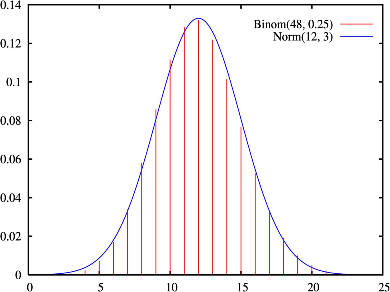
Counts follow a binomial distribution, which is lumpy and discrete. But when n is big enough, that binomial histogram is well approximated by a smooth normal curve — exactly what the figure above shows — and the normal-curve machinery from Section 2 applies again. The standard error of a sample proportion works out to √[p(1 − p)/n], and since p is the very thing we do not know, we substitute p̂:
p̂ ± z* · √[p̂(1 − p̂)/n]
Note that this one uses z, not t. There is no separate standard deviation to estimate here: for a yes/no variable, the proportion is the mean and it determines the variability all by itself, so there is no extra degrees-of-freedom correction to make.
The conditions — check them first
This formula is an approximation, and it is a bad one when the sample is small or the proportion is close to 0 or 1. Three conditions protect you.
| Condition | How to check | Why it matters |
|---|---|---|
| Random sample | The data came from random selection or random assignment | Without it the estimate is biased, and no formula can repair bias |
| Independence (10% rule) | n < 10% of the population when sampling without replacement | Keeps the standard error formula valid |
| Success-failure | np̂ ≥ 10 and n(1 − p̂) ≥ 10 | At least ~10 of each outcome, or the binomial is too skewed for a normal curve |
Worked example. In a random sample of n = 400 adults, x = 148 say they exercise regularly. Build a 95% confidence interval for the population proportion p.
- Point estimate: p̂ = 148/400 = 0.37
- Conditions: np̂ = 400(0.37) = 148 ≥ 10 ✓ and n(1 − p̂) = 400(0.63) = 252 ≥ 10 ✓
- Standard error: √[(0.37)(0.63)/400] = √(0.2331/400) = √0.00058275 = 0.02414
- Critical value: z* = 1.96
- Margin of error: 1.96 × 0.02414 = 0.0473, or 4.7 percentage points
- Interval: 0.37 − 0.047 = 0.323 and 0.37 + 0.047 = 0.417
The 95% confidence interval is 0.323 to 0.417, or roughly 32% to 42%. This is exactly the kind of interval a news outlet compresses into “37%, plus or minus about 5 points.”
Percentage points are not percent
When a result is itself a percentage, language gets slippery. A margin of error of 4.7 percentage points means the endpoints are 32.3% and 41.7%. It does not mean 4.7% of 37%, which would be a margin of only 1.7 points. Always say “percentage points” when you mean an additive move on a percentage scale — the distinction shows up in polling coverage, quality reporting, and clinical trial write-ups alike.
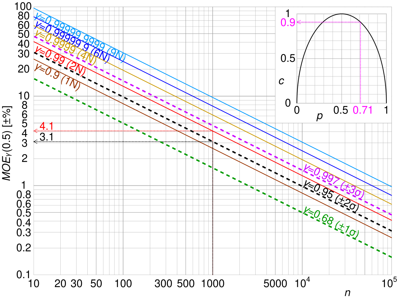
One more practical note. Political polls typically publish a single “margin of error” computed at the most conservative case, p̂ = 0.5, because that is where p̂(1 − p̂) is largest. That is why a poll of 1,000 people is nearly always described as ± 3 points regardless of what the actual percentages came out to.
- For a proportion: p̂ ± z*√[p̂(1 − p̂)/n], using z rather than t.
- Check random sampling, the 10% independence rule, and the success-failure condition (np̂ ≥ 10 and n(1 − p̂) ≥ 10).
- Report the margin in percentage points, not as a percent of the estimate.
- Variability is largest at p̂ = 0.5, which is why published poll margins assume that worst case.
Section 4Margin of error and sample size
The three dials
Because the margin of error is a critical value times a standard error, only three things can change an interval's width, and each behaves in a predictable way.
Confidence level. Raising confidence raises the critical value, so the interval gets wider. This is not a defect; it is the price of a stronger guarantee. If you want to be right almost every time, you must say something vaguer. At the extreme, a 100% confidence interval for average sleep would be “between 0 and 24 hours” — certainly correct and completely useless.
Sample size. Increasing n shrinks the standard error, so the interval gets narrower. But the √n in the denominator sets the exchange rate, and it is a harsh one: to halve the margin of error you must quadruple the sample size. Doubling n only buys you a factor of 1/√2 ≈ 0.71.
Variability. More spread in the population (a larger σ or s) means a larger standard error and a wider interval. You usually cannot change this one — it is a property of the world, not of your study — though careful measurement and homogeneous subgroups can reduce it.
| Change | Critical value | Standard error | Margin of error | Interval |
|---|---|---|---|---|
| Confidence 90% → 99% | 1.645 → 2.576 (up) | unchanged | up | Wider |
| Confidence 99% → 90% | 2.576 → 1.645 (down) | unchanged | down | Narrower |
| Sample size n × 4 | unchanged (roughly) | ÷ 2 | ÷ 2 | Half as wide |
| Sample size n ÷ 4 | unchanged (roughly) | × 2 | × 2 | Twice as wide |
| Population more spread out | unchanged | up | up | Wider |
Seeing the dials turn
Return to the reaction-time sample: x̄ = 78.4, s = 9.0, n = 25, df = 24, standard error 1.80. Hold the data fixed and turn only the confidence dial.
| Confidence | t* (df = 24) | Margin of error | Interval | Width |
|---|---|---|---|---|
| 90% | 1.711 | 1.711 × 1.80 = 3.08 | 75.32 to 81.48 | 6.16 |
| 95% | 2.064 | 2.064 × 1.80 = 3.72 | 74.68 to 82.12 | 7.44 |
| 99% | 2.797 | 2.797 × 1.80 = 5.03 | 73.37 to 83.43 | 10.06 |
Now hold confidence at 95% and turn only the sample-size dial, treating the standard deviation as a known σ = 9.0 so the multiplier stays fixed at 1.96:
| Sample size n | Standard error 9/√n | Margin of error (1.96 × SE) | Interval about x̄ = 78.4 |
|---|---|---|---|
| 25 | 9/5 = 1.80 | 3.53 | 74.87 to 81.93 |
| 100 | 9/10 = 0.90 | 1.76 | 76.64 to 80.16 |
| 400 | 9/20 = 0.45 | 0.88 | 77.52 to 79.28 |
Each fourfold jump in n cuts the margin exactly in half. Going from 25 to 400 participants — sixteen times the data collection — buys a margin one quarter as large.
Planning a study: solving for n
Turn the formula around and you get a planning tool. Decide the margin of error E you can live with, pick your confidence level, and solve.
For a mean. From E = z*σ/√n, solving gives n = (z*σ/E)2. Suppose a pilot study suggests σ ≈ 12 and you want a 95% interval with margin no larger than 2 points.
- n = (1.96 × 12 / 2)2 = (11.76)2 = 138.3
- Always round up: recruit 139 participants.
For a proportion. From E = z*√[p(1−p)/n], solving gives n = z*2p(1−p)/E2. If you have no prior estimate of p, use p = 0.5, which maximizes p(1−p) at 0.25 and therefore gives the safest (largest) answer. For a 95% interval with a margin of 3 percentage points:
- n = (1.96)2(0.25)/(0.03)2 = 3.8416 × 0.25 / 0.0009
- = 0.9604 / 0.0009 = 1067.1
- Round up: survey 1,068 people.
That number should look familiar. It is why national polls so consistently sample around a thousand respondents: roughly a thousand people buys a 3-point margin, and pushing to 1 point would require about 9,600.
- Higher confidence → larger critical value → wider interval; there is no free lunch.
- Larger n → smaller standard error → narrower interval, but only at rate 1/√n: quadruple n to halve the margin.
- For a mean, n = (z*σ/E)2; for a proportion, n = z*2p(1−p)/E2, using p = 0.5 when nothing is known.
- Always round the required sample size up to the next whole person.
Section 5Interpreting a confidence interval correctly
The sentence that is right
Here is a template you can use every time, and it is worth writing down word for word:
“We are 95% confident that the interval from 74.68 to 82.12 contains the true mean reaction-time score for the population.”
Three ingredients make it correct: the confidence level, the interval, and a clear statement of the parameter in context — whose mean, of what, measured how. Drop any one of them and the sentence loses its meaning.
And what does the 95% attach to? Not to this interval. It attaches to the procedure. Imagine repeating the whole study — draw a fresh random sample, compute x̄ and s, build the interval — over and over, thousands of times. Each repetition gives a different interval, centered somewhere slightly different, with a slightly different width. In the long run, about 95% of those intervals will contain the true μ, and about 5% will miss it entirely. That long-run success rate is the coverage probability, and it is the only thing 95% ever meant.
The catch is that you built exactly one interval, and you cannot tell whether yours is one of the 95% or one of the 5%. Your interval either contains μ or it does not. There is no partial credit and no randomness left to describe: μ is a fixed number, and your endpoints are now fixed numbers too.
The four sentences that are wrong
Each of the following is a real thing students, journalists, and occasionally published researchers write. Each is wrong, and it is worth knowing precisely why.
| Wrong statement | Why it fails | What it should say |
|---|---|---|
| “There is a 95% probability that μ lies in this interval.” | μ is a fixed constant and the endpoints are now fixed numbers; the probability is 0 or 1, we just do not know which. The 95% describes the long-run procedure. | “95% of intervals built this way capture μ.” |
| “95% of the data values fall between 74.68 and 82.12.” | Confuses the spread of individuals with the precision of an estimate. An interval for a mean is usually far narrower than the data. | “This interval estimates the mean, not the range of scores.” |
| “95% of future sample means will fall in this interval.” | Future sample means vary around μ, not around your particular x̄; the actual capture rate for that claim is well under 95%. | “The interval estimates μ, not the location of future samples.” |
| “The interval contains 80, so we have proved μ = 80.” | An interval lists plausible values, all of them at once. 74.7 is just as much ‘in’ the interval as 80 is. | “80 is a plausible value for μ; so is every other number in the interval.” |
A fifth error deserves its own mention because it travels with confidence intervals so often. A p-value is not the probability that the null hypothesis is true — it is the probability of observing data at least as extreme as yours assuming the null hypothesis is true. Confidence intervals and p-values are two views of the same calculation, and they inherit the same discipline: both are statements about how data behave under a hypothesis, never statements about how likely a hypothesis is.
The same discipline governs the language of decisions. When an interval contains a claimed value — equivalently, when the corresponding test does not reach significance — the correct phrase is fail to reject, never accept. Failing to reject means only that the data were consistent with that value, not that the value is true: the interval 74.68 to 82.12 is exactly as consistent with 80 as it is with 74.7 or 82.1, and it cannot single one of them out. Absence of evidence against a value is not evidence for it, and a wide interval usually means you had too little data to distinguish anything at all.
What an interval is genuinely good for
Used correctly, a confidence interval does three jobs a single p-value cannot. It shows the size of the effect, not just whether one exists. It shows the precision of your estimate through its width — a narrow interval around a small effect and a huge interval around a large one tell very different stories. And it supports a quick significance check: if a 95% interval for a difference does not contain 0, the corresponding two-sided test rejects at α = 0.05; if a 95% interval for a mean does not contain 80, a two-sided test of μ = 80 rejects at α = 0.05.
Finally, keep the interval's scope honest. A margin of error quantifies random sampling variation only. It does not cover a biased sampling frame, people who refused to answer, a leading question, a miscalibrated instrument, or data entered wrong. Those errors can dwarf the margin of error, and no amount of extra sample size will shrink them — more data collected badly just gives you a tighter interval around the wrong number.
- Correct form: “We are C% confident that the interval (a, b) contains the true parameter in context.”
- The confidence level describes the long-run procedure — about 95% of intervals built this way capture the parameter.
- A CI is not about data values, not about future sample means, and does not assign probability to a fixed μ.
- A value inside the interval is plausible, not proven; “fail to reject” never means “accept.”
- Margin of error covers random sampling variation only — never bias, non-response, or measurement error.
The chapter in one breath
- A point estimate is a single best guess; because of sampling error it is almost certainly a little wrong, so we report a range instead.
- Every confidence interval is point estimate ± (critical value × standard error), and the width of the interval is twice the margin of error.
- For a mean with σ known, use x̄ ± z*(σ/√n); with σ unknown use x̄ ± t*(s/√n) with df = n − 1.
- The t distribution has heavier tails to pay for estimating σ, and converges to z as n grows; at 95%, z* = 1.96.
- For a proportion, use p̂ ± z*√[p̂(1−p̂)/n] after checking random sampling, the 10% rule, and success-failure (at least 10 of each outcome).
- Higher confidence widens the interval; larger n narrows it only at rate 1/√n, so quadrupling n halves the margin.
- To plan a study, solve n = (z*σ/E)2 for a mean or n = z*2p(1−p)/E2 for a proportion, use p = 0.5 when in doubt, and always round up.
- “95% confident” describes the long-run procedure, not a probability for this one interval — and the margin of error covers random variation only, never bias.
ReferenceWords worth knowing
A quick reference for the vocabulary in this chapter — skim it now, then circle back whenever a term in a formula or an interpretation stops making sense.
- Central Limit Theorem
- The result that, for a large enough sample, the sampling distribution of x̄ is approximately normal regardless of the population's shape. It is what licenses the normal-curve critical values used in these intervals.
- Confidence interval
- An interval estimate for a population parameter, computed as point estimate ± margin of error and reported with a confidence level.
- Confidence level
- The long-run percentage of intervals built by a given procedure that would capture the true parameter; common choices are 90%, 95%, and 99%.
- Coverage probability
- The actual long-run proportion of intervals from a procedure that contain the parameter. A good procedure has coverage close to its stated confidence level.
- Critical value
- The multiplier (z* or t*) applied to the standard error, chosen from a distribution table to match the desired confidence level.
- Degrees of freedom (df)
- The parameter that selects which t curve to use; for a one-sample interval for a mean, df = n − 1.
- Interval estimate
- A range of plausible values for a parameter, as opposed to a single number.
- Margin of error
- The half-width of a confidence interval: critical value × standard error. It quantifies random sampling variation only.
- Parameter
- A fixed numerical fact about a whole population, such as μ or p. It is unknown and does not vary from sample to sample.
- Point estimate
- A single-number estimate of a parameter computed from sample data, such as x̄ for μ or p̂ for p.
- Population proportion (p)
- The true fraction of the population with a given characteristic — the parameter estimated by p̂.
- Prediction interval
- An interval intended to contain a future individual observation rather than a parameter; it is always wider than a confidence interval for the mean.
- Sample proportion (p̂)
- The fraction of successes in the sample, x/n; the point estimate for p.
- Sampling distribution
- The distribution of a statistic's values across all possible samples of a given size. Its standard deviation is the standard error.
- Sampling error
- The natural sample-to-sample variation of an estimate. It is not a mistake, and it is the only thing a margin of error accounts for.
- Standard error
- The standard deviation of a statistic's sampling distribution — σ/√n or s/√n for a mean, √[p̂(1−p̂)/n] for a proportion.
- Statistic
- A number computed from sample data, such as x̄, s, or p̂. Unlike a parameter, it varies from sample to sample.
- Student's t distribution
- A family of symmetric, bell-shaped curves with heavier tails than the normal, indexed by degrees of freedom; used when σ must be estimated by s.
- Success-failure condition
- The requirement np̂ ≥ 10 and n(1 − p̂) ≥ 10 that makes the normal approximation to the binomial adequate for a proportion interval.
- t critical value (t*)
- The multiplier taken from the t distribution with n − 1 degrees of freedom; at 95% it is 2.064 for df = 24 and shrinks toward 1.96 as df grows.
- Width
- The full length of a confidence interval, upper endpoint minus lower endpoint — exactly twice the margin of error.
- z critical value (z*)
- The multiplier taken from the standard normal curve: 1.645 for 90%, 1.960 for 95%, and 2.576 for 99% confidence.